TIL corner turning in GPUs
(NOTE: this isn’t my best work, and its still kinda WIP, so expect inaccuracies and incomplete parts.)
I’ve working my way through Programming Massively Parallel Processors. There’s many interesting bits of knowledge I’ve learned about GPUs, and the bit I want to write down is called ‘corner turning’. It took me a while to wrap my head around it, so I hope this post will serve me well when I need to come back and relearn it at some point in the future.
Before we get to corner turning, we need to briefly talk about the basics of GPU architecture and the concept of ‘tiling’ when programming stuff to run on a GPU.
GPU Architecture
I’m going to try and keep things very simple here. A GPU is composed of many streaming multiprocessors (SMs). Each multiprocessor has several cores.
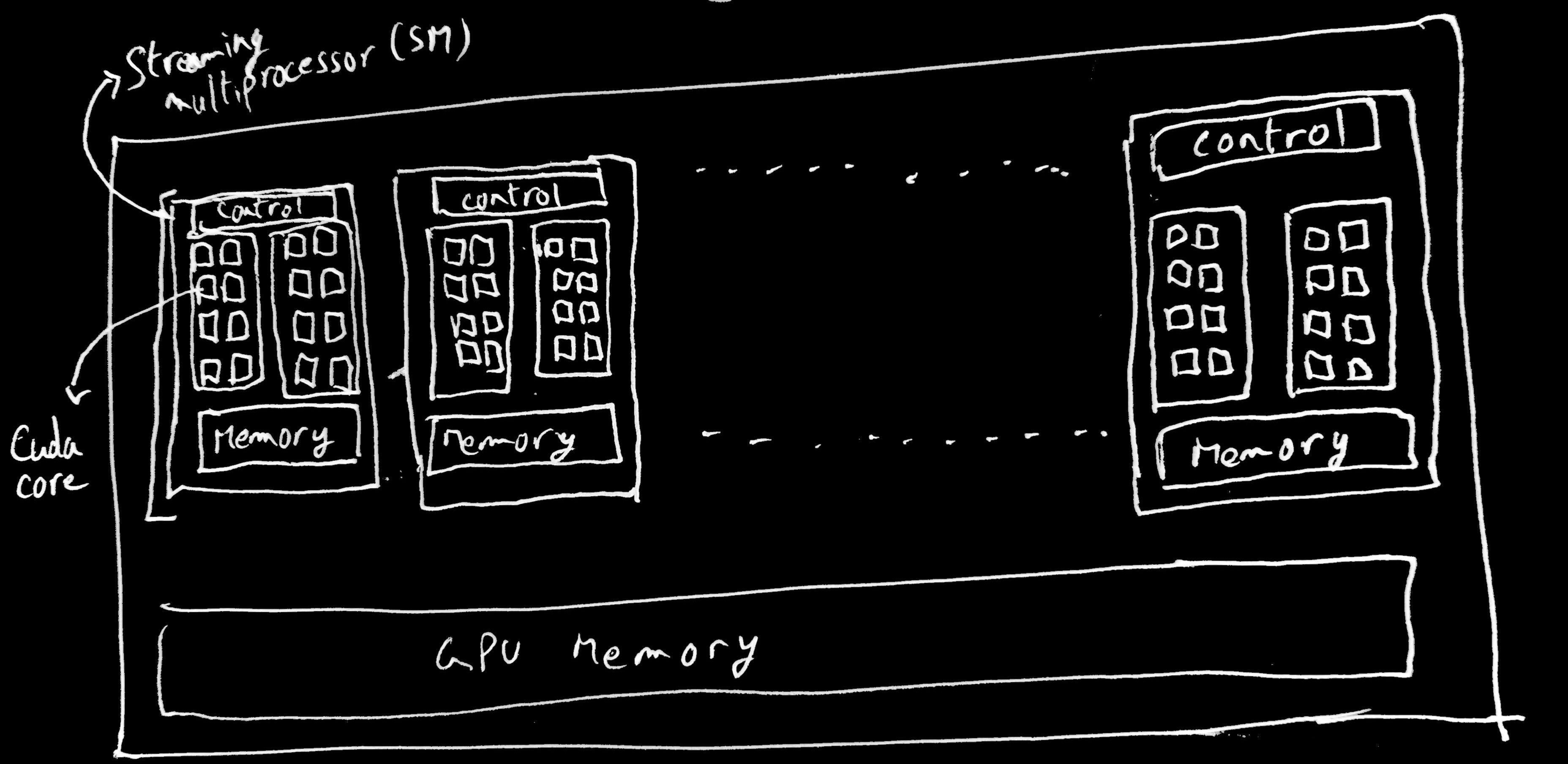
In order to run something on a GPU, you write a function (called a ‘kernel’ in GPU programming land, not to be confused with kernels of operating systems). This function is then “launched” by a call to that function with some special parameters.
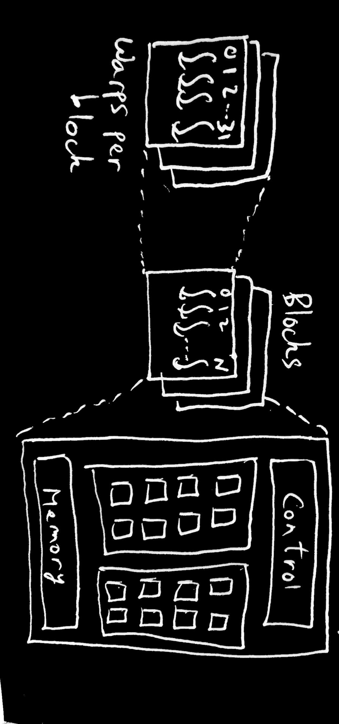
This kernel launch specifies the number of threads that will be executing this function. The threads are organized into “blocks”. A collection of these blocks is called a “grid”. For ease of addressing individual threads in a grid, you can can organize your blocks in 1, 2, or 3 dimensions depending on what makes sense for working with your data. The same applies for organizing the threads in the block. Depending on the particular GPU you are using, there are upper limits on the number of blocks and threads and the dimensions of your grid and blocks.
// This is a kernel that takes pointers to three arrays on the GPU, adds the
// elements of A and B and places the result in C.
// Each thread launched executes
// this same code. The `id` value is based on the thread id and the block id.
// blockIdx, blockDim, threadIdx values are determined by the kernel launch
// parameters.
// This is a common pattern where the id of the thread is used to determine
// which subset of the data it operates on. So in this case, each thread will
// calculate one result in the output array.
#define N 4096
__global__ void vecadd(int *A, int *B, int *C) {
  int id = blockIdx.x * blockDim.x + threadIdx.x;
  if (id < N) {
    C[id] = B[id] + A[id];
  }
}
int main {
  // ... other stuff

  // This 'launches' the kernel with 4096 threads, divided into blocks of
  // 256 threads (so 4 blocks). The two parameters inbetween <<< and >>>
  // are the grid size and block size respectively. The threads are organized in
  // 1D in this example, but can be up to 3D.
  vecadd<<<N / 256, 256>>>(A_d, B_d, C_d);

  // .. other stuff
}
All the threads in a given block will be scheduled onto the same SM (this is necessary for various reasons, one of which is that a block can also have a small shared memory pool in the SM itself that it can use for fast data access and for coordinating the threads. An SM itself can have multiple blocks. It’s just that blocks cannot be spread over multiple SMs). These threads are SIMD, so they all expect to perform the same task at each step, with different data units that is fed to each thread. When threads in a block are actually scheduled to run on the cores in the SM, they are scheduled in groups of 32 threads in Nvidia GPUs (called warps) or groups of 64 in AMD GPUs (called wavefronts). The nitty gritty details of how the scheduling of threads in a warp onto the hardware is actually done isn’t important for this post. Just know that a thread is executing an instruction, 31 of its neighboring peers are executing the same instruction at that moment. So if a thread is executing a load instruction where its loading some data from memory into its local register, the other threads in the warp are doing the same thing (for the data assigned to that particular thread. Remember its SIMD). The hardware is clever enough to check if all the threads in the warp or wavefront are loading data that are adjacent to each other in memory. And if they are, then it can coalesce the memory accesses of the threads in the warp into one request to the RAM. This speeds up your code because you’re cutting down on the number of memory accesses being performed. Remember this point because it is relevant to why corner turning is useful.
Tiling
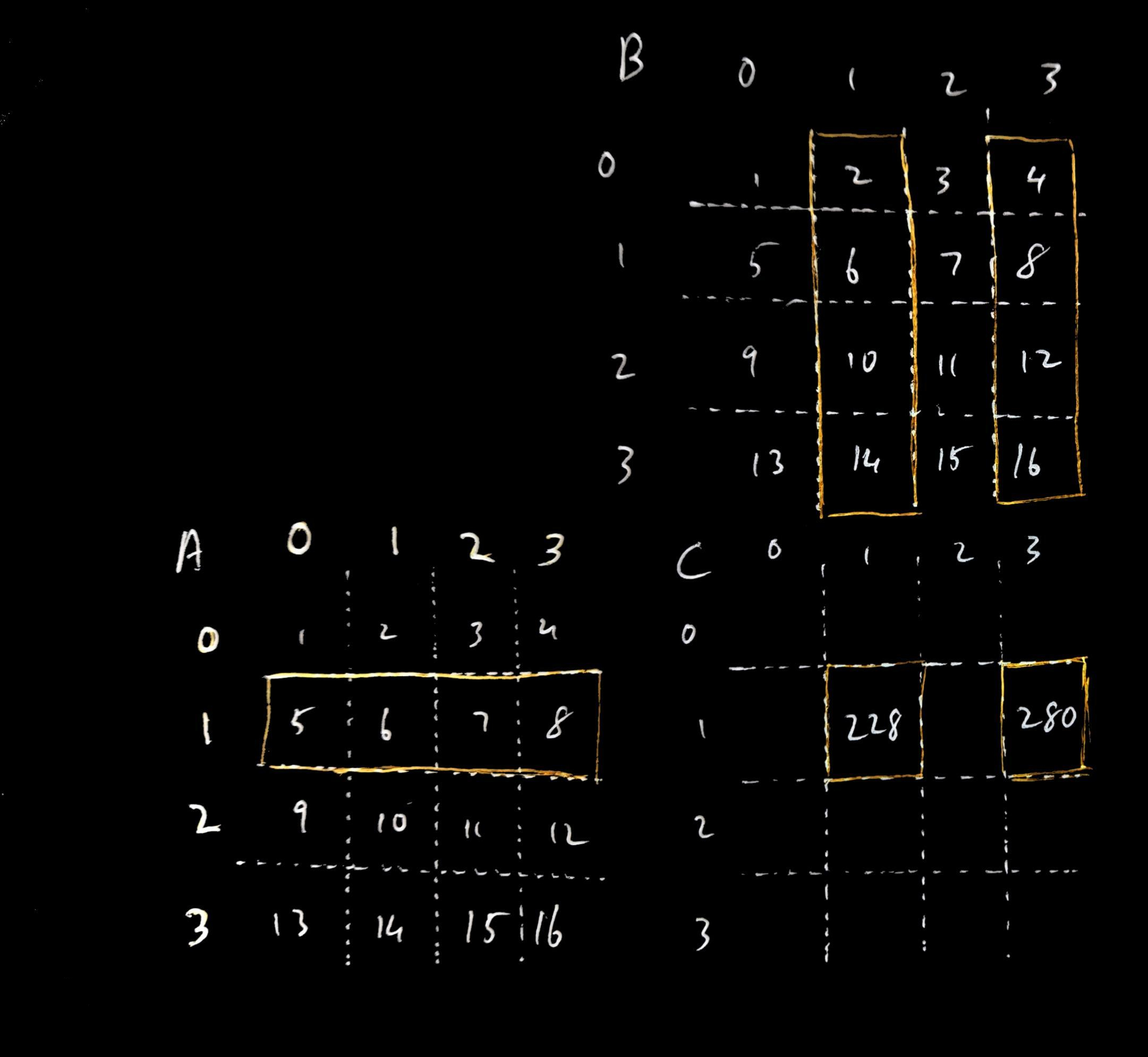
A naive algorithm for matrix multiplication is one where you set up block and grid size such that there is one thread for each element of the output matrix. So that thread will be responsible for reading the corresponding row and column of the input matrices, calculating the dot product, and writing the output into the output matrix. The thing is, multiple threads might be reading the same row or same column as other threads to calculate their output element.
For example, if you are multiplying two 4x4 matrices A and B, your output matrix C is also 4x4. If you look at output element C11 and C13 (the element on row 1, column 1 and the element on row 1, column 3), both these values require the entirety of row 1 of matrix A. If the value of C11 and C13 are being calculated by separate threads working completely independently of each other, they will make redundant memory accesses to the same row 1 of matrix A.
Every block has access to a shared memory area (sometimes called local data store or LDS) that it can use to coordinate its threads. If if the threads in a block were able to work together, they could load and share the data they all need in the LDS, cutting down on redundant memory accesses. One technique that does this is called ‘tiling’ since a ‘tile’ (a small section of the input matrix usually the same dimensions of the thread block) is loaded into the LDS for each input matrix, the threads in the block calculate the partial dot product from the data in the LDS, then load the next tile needed by the block into the LDS until each thread has calculated its final output.
As an example, lets say we have our 4x4 input matrices A and B, and multiply them to produce our output matrix C. Let’s say we launch our matrix multiplication kernel with 4 2x2 blocks, and the grid of blocks also 2x2 dimensions. We can divvy up the work such such each output element of C is calculated by a unique thread e.g. element C00 is calculated by thread t00 in block b00, element C31 is calculated by thread t10 in block b10, and so on. You can also see that each block of threads is calculating the output elements of a particular output ‘tile’ in C i.e. a subset of the output matrix.
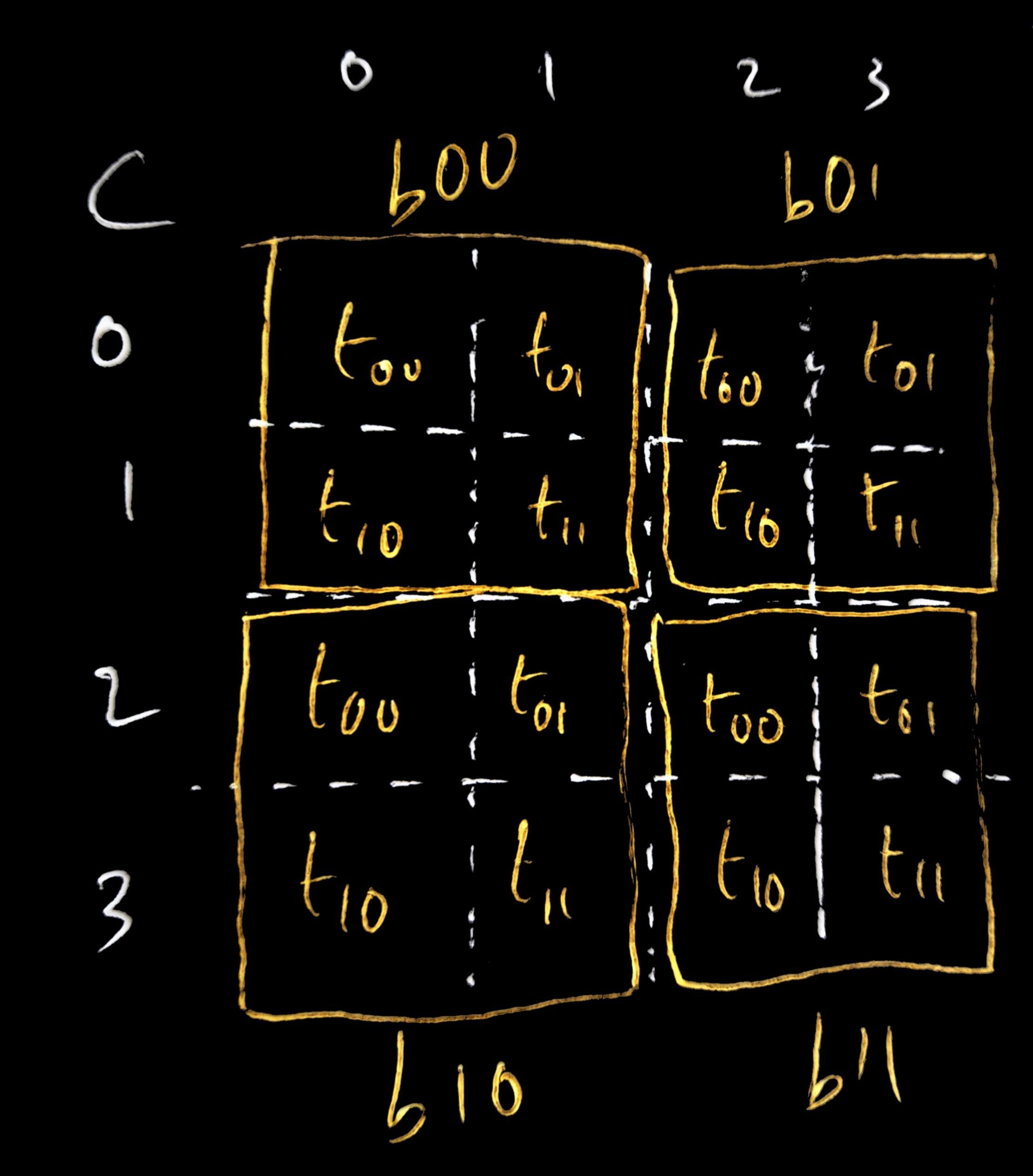
Continuing our example, lets look at the tile calculated by block b11 (the
bottom right tile). The output values in the b11 tile in matrix C are calculated by
using the rows 2 and 3 from matrix A and columns 2 and 3 from B. We can see, for
example, that both outputs C22 and C23 (calculated by t0 and t1 in B11) require the
elements A20 and A21 when calculating the output. If t0 and t1 were working
independently, they would both separately make the same (slow) read request to RAM to load
A20 and A21. In tiling, we would instead have t00 and t01 load A20 and A21
respectively and store them in the block b11’s LDS so that they both can access those
input elements from the fast LDS. This saves the redundant memory accesses. Similarly, t10 and t11
will respectively load A30 and A31 into the LDS so that both threads have fast
access to it. A similar
load is done by b11 for the input matrix B, loading B02, B03, B12, B13 by
the corresponding threads into the LDS. With the tiles loaded, each thread in
the block calculates the partial dot product from the input elements available
in the LDS (t00 calculates A20*B02+A21*B10, t01 calculates A20*B03+A21*B13
and so on), and stores the partial dot product in thread local storage (since, remember, each thread
is assigned to calculate one output element of C, so we don’t need LDS for the output elements). The block then moves to load the next tile from the input elements
(A22, A23, A32, A33 from A; B22, B23, B32, B33 from B; each respectively loaded
by t00, t01, t10, t11). With the new tiles in LDS, the partial dot product is
calculated again by each thread for its assigned output element and this is
summed with the previous dot product the thread had calculated to get the final
output.
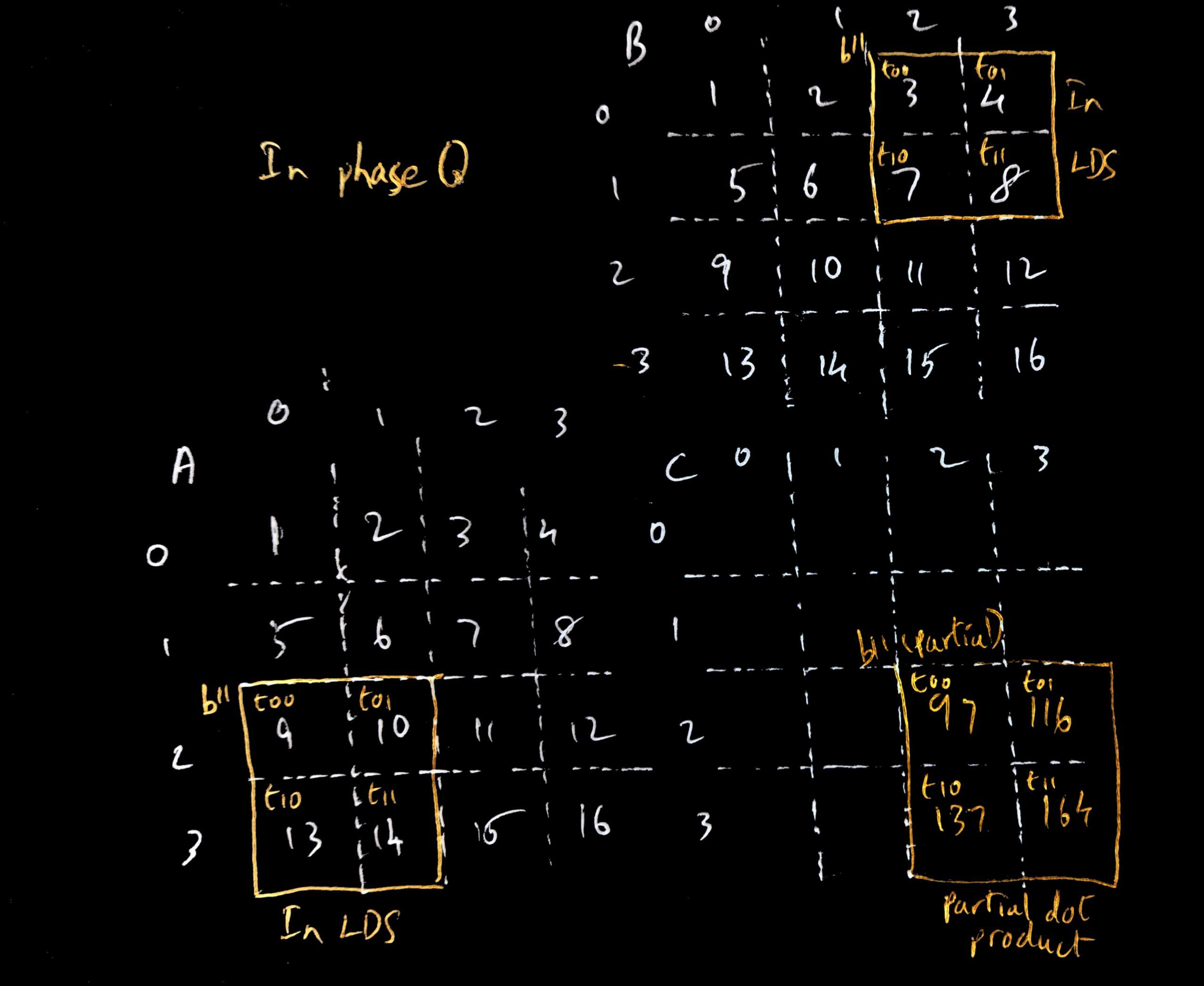
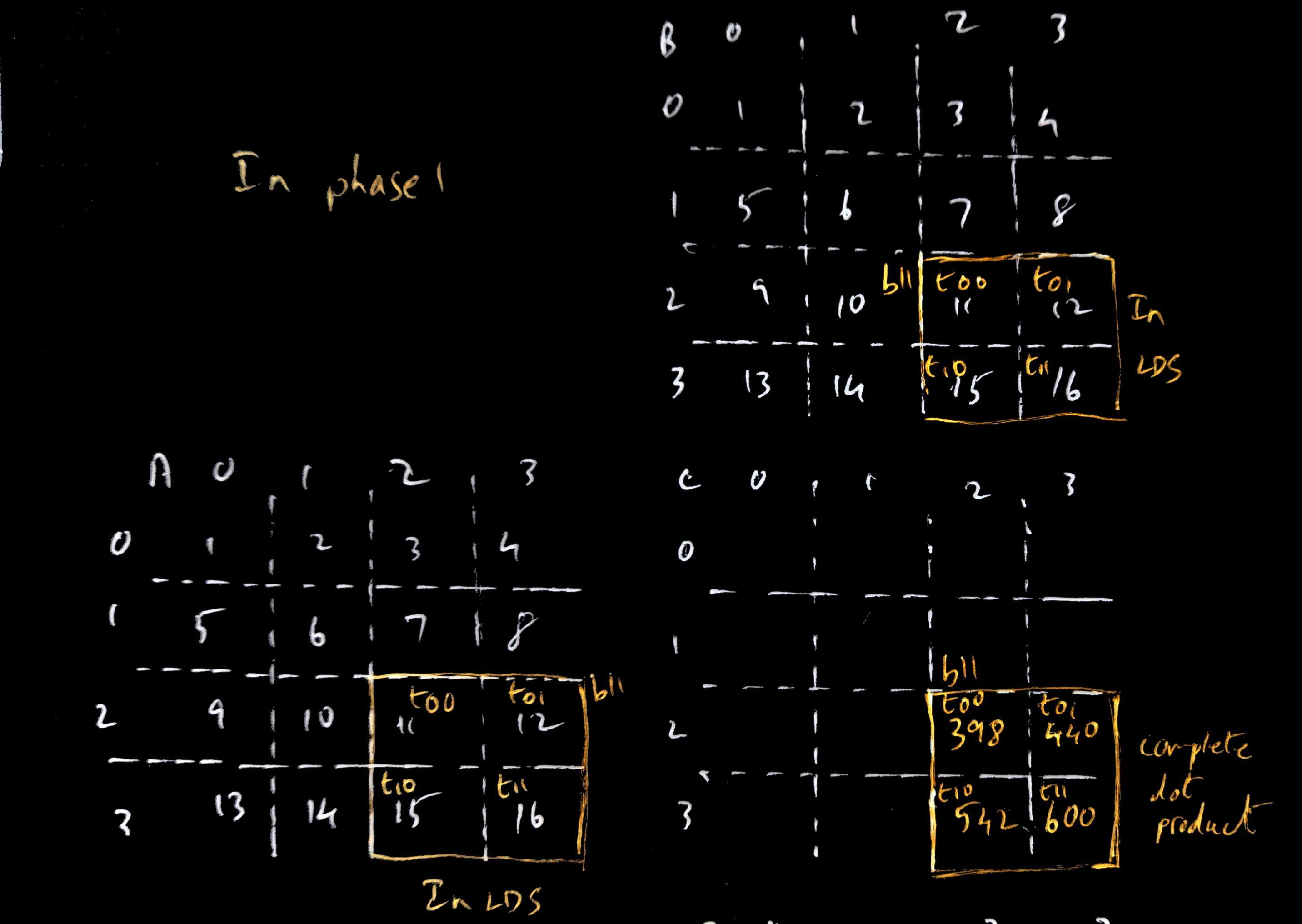
This process of loading tiles in phases and calculating the partial dot product in each phase is being done by each of the other blocks as well.
If the threads in b11 weren’t working together in this way, t00 for example would’ve made 4 memory accesses to read row 2 from matrix A. With 2x2 tiles, it only needed to make 2. In general, the number of total memory accesses being done is reduced by a factor N if your tile is NxN elements.
See here for an example showing matrix multiplication with tiling
The part of the code to focus on is the kernel which shows how the kernel sets up the LDS for the block to store tiles for the input matrices. And then in a loop - the tile from each input matrix is loaded by the block, the partial dot product is calculated by each thread in the block, and then the next tile is loaded to continue the process.
Corner Turning
Now tiling is a pretty good optimization by itself. Everything we talked about above assumes your matrices are stored in memory in row major order. This means that in memory, the elements of a matrix are stored in 1D (because addressing in RAM is one dimensional), and they are arranged such that the first row is arranged in sequence, followed by the second row, and so on. q
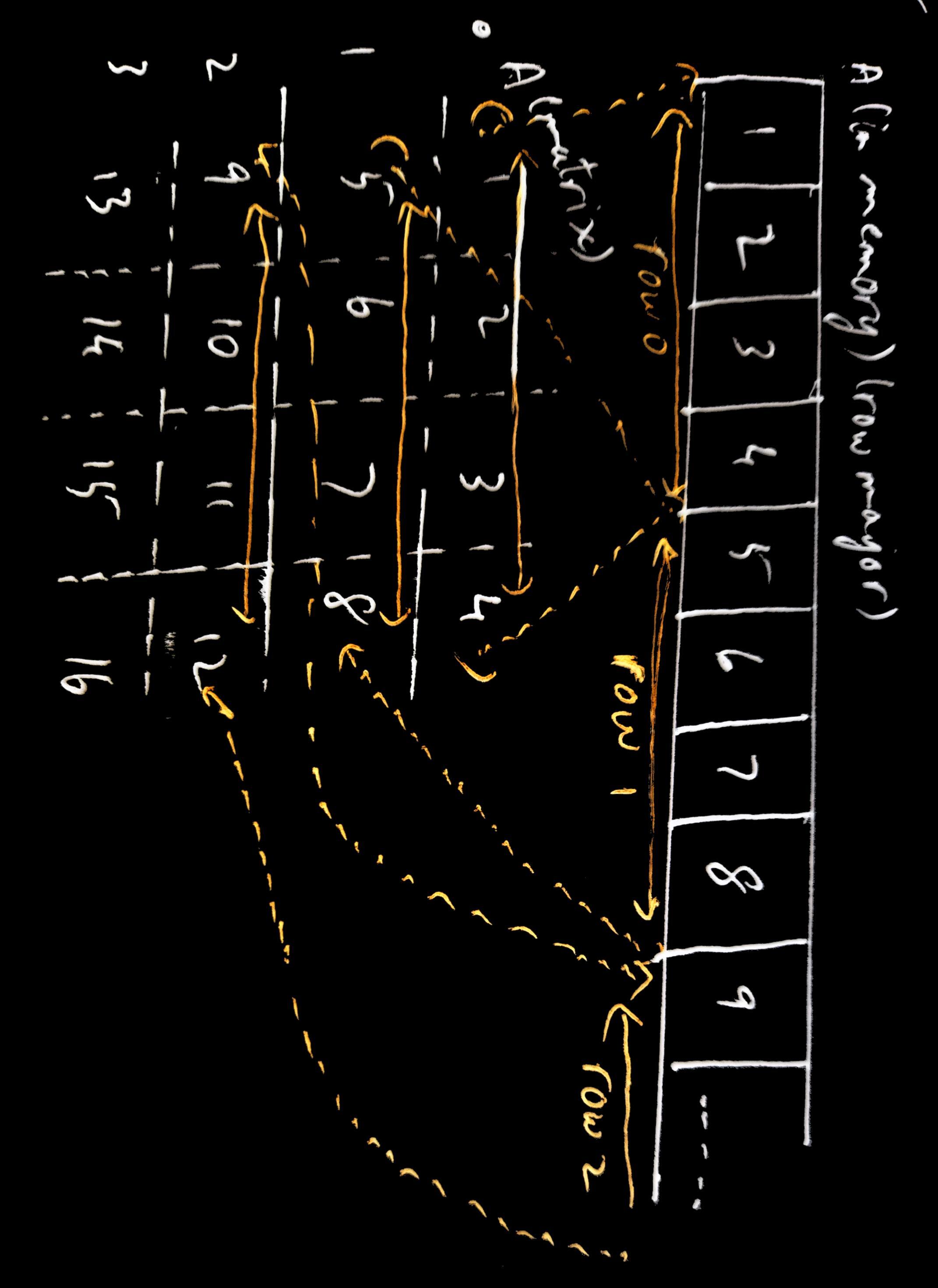
Corner turning is a further optimization you can make when one of your input matrices is in column major order.
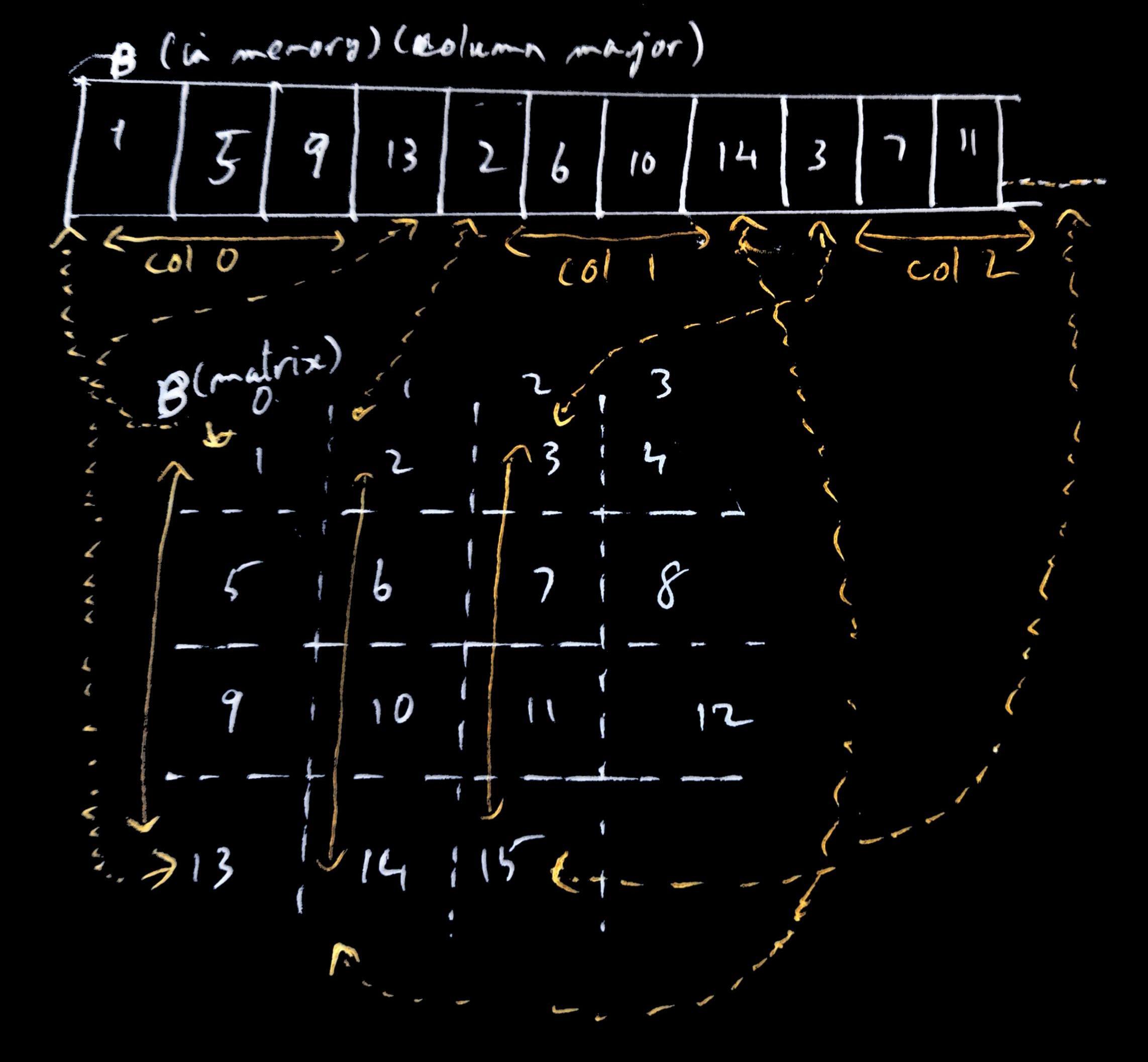
Remember we talked earlier how threads are scheduled in the hardware in groups of 32 or 64 neighboring threads called warps or wavefronts. And how since they are SIMD they all perform a load instruction at the same time, and the hardware can try to coalesce the memory accesses into one if they are accessing data that is adjacent to each other. In the normal way we load a tile into LDS for a matrix that’s in row major order, threads next to each other are loading data that are next to each other in memory.
Say our matrix A is much larger and we are using 4x4 tiles (so each block of
threads has 4x4 threads). Lets imagine just for the purpose of this explanation our warp size is 4
i.e. threads are scheduled on the hardware in groups of 4 threads. When we load a tile and the matrix is in row major
order, adjacent threads are loading data that is adjacent in memory.
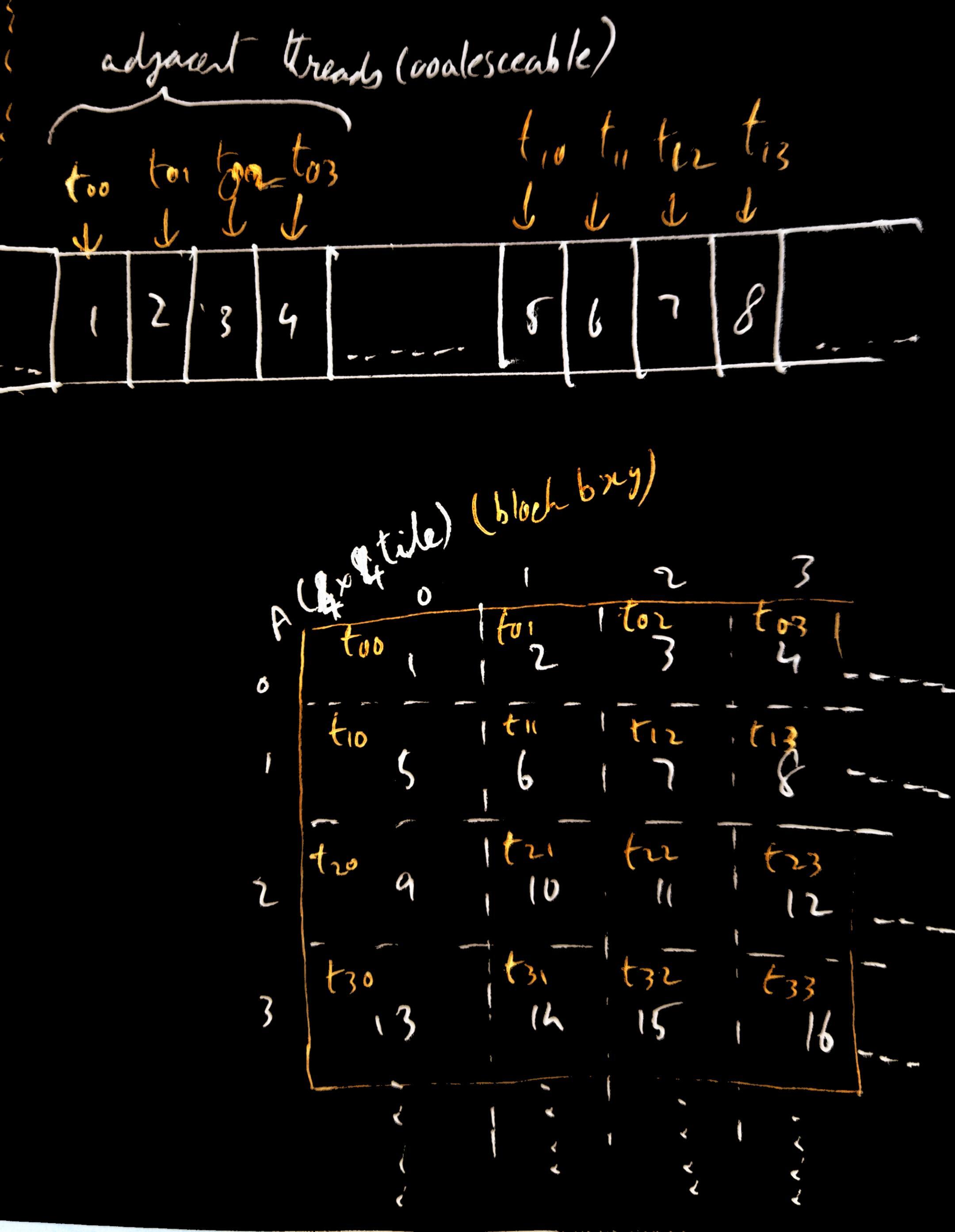 In the diagram above, t00, t01, t02, t03 are adjacent threads in a block and
are scheduled together in the warp. They are loading adjacent elements in
memory into the LDS, so the memory requests of the threads can be coalesced
into one request, cutting down the number of memory operations.
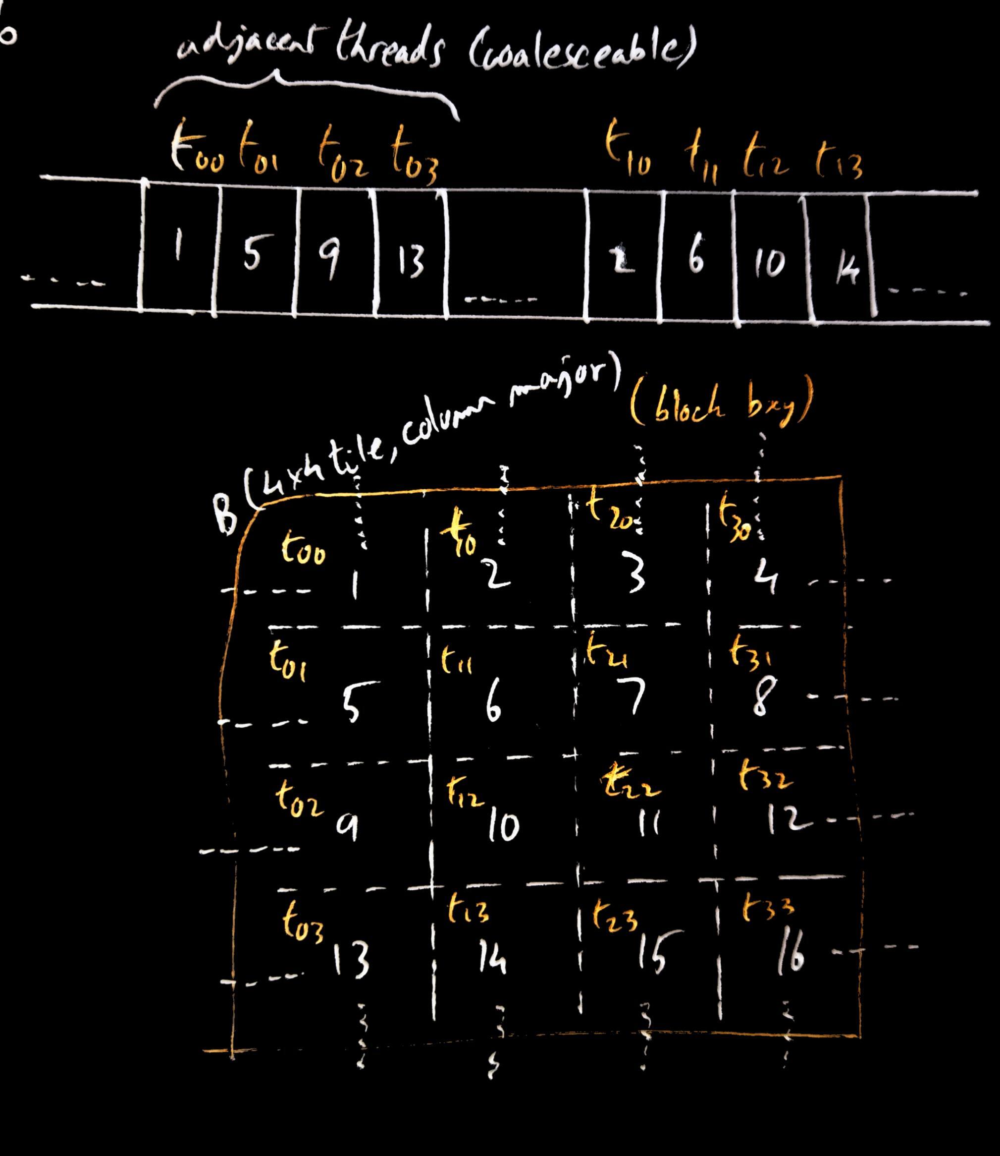
But when the matrix is in column major order, but the threads in a block are still assigned to load along the rows of a tile, adjacent threads are not loading data next to each other. So when they are scheduled together in a warp, the hardware can’t coalesce the memory access request leading to more overall memory accesses.

In the diagram above, we see that threads t00, t01, t02, t03 are loading elements that are far away from each other in memory because the threads are trying to load elements along the row of the tile, but in memory the elements of the tile’s row are far away from each other due to the column major order in which the matrix was stored. Since the threads t00 to t03 are scheduled as a warp but the elements are far away from each other in memory, the memory requests cannot be coalesced, so the number of memory accesses is higher.
To solve this, adjacent threads in the block are made to load data along the column of the tile instead of along the row. And since the matrix is in column major order, the elements in the column of the tile are adjacent to each other in memory, so when a warp is scheduled and the neighboring threads are loading the data along the column, the hardware can coalesce the request.
The problems
The example codes linked in the previous section run a benchmark where the kernel is run 150 times, and the mean time is calculated. Ostensibly, the corner turning method should be universally faster than not corner turning, when given two matrices M and N where N is in column major order (and corner turning is either applied or not applied when loading tiles from N). But when I actually ran the benchmark on different GPUs, they produce conflicting results.
| GPU | Corner turning | Mean Time (ms) |
|---|---|---|
| Nvidia 4090 (10000 width matrix) | With Corner Turning | 1469.3 |
| Nvidia 4090 (10000 width matrix) | Without Corner Turning | 1568.08 |
| Nvidia V100 (30000 width matrix) | With Corner Turning | 19378.8 |
| Nvidia V100 (30000 width matrix) | Without Corner Turning | 18579.8 |
| AMD MI250X (30000 width matrix) | With Corner Turning | 16865.9 |
| AMD MI250X (30000 width matrix) | Without Corner Turning | 14489.7 |
I can’t for the life of me figure out why corner turning has a speed up on my 4060 but is slower than no corner turning on a V100 and an MI250X. So that’s still something to figure out.